Data Visualization with PIC GUI
Overview
PIC GUI is a lightweight, user-friendly data visualization tool that enables real-time monitoring of variables from your embedded application. Unlike External Mode (which requires XCP protocol), PIC GUI provides a simplified approach to streaming data over UART for analysis and debugging.
PIC GUI vs External Mode
| Feature | PIC GUI | External Mode |
|---|---|---|
| Communication Protocol | Simple UART packet format | XCP protocol over Serial/TCP/UDP |
| Setup Complexity | Very Simple | - Drag UART Tx-Matlab block, configure baud rate |
| Data Monitoring | Yes | - Stream variables to MATLAB for plotting |
| Parameter Tuning | No - Read-only data streaming | Yes |
| Synchronization | Asynchronous data logging | Synchronized with Simulink simulation time |
| Custom Visualization | Yes | - Full MATLAB scripting for custom plots/analysis |
| Typical Use Case | Data logging, debugging, custom analysis | Interactive parameter tuning, live scope monitoring |
| Hardware Requirements | UART peripheral + USB-Serial adapter | UART/Ethernet/CAN + XCP support |
When to Use Each Tool:
- Use PIC GUI when you need quick data logging, custom MATLAB analysis, or read-only monitoring
- Use External Mode when you need to tune parameters in real-time or require synchronized scope displays
- Use Both - They can coexist! Use External Mode for tuning, PIC GUI for detailed data analysis
How PIC GUI Works
Data Flow
- Embedded Side: UART Tx-Matlab block packages selected variables into packets and transmits via UART
- Serial Connection: USB-Serial adapter bridges microcontroller UART to PC COM port
- MATLAB Side: PIC GUI decodes packets and makes data available as MATLAB variables
- Visualization: Custom MATLAB script plots data in real-time or saves for offline analysis
Packet Format
The UART Tx-Matlab block uses a simple, efficient packet structure:
- Start Byte: Synchronization marker (0x5A)
- Data Length: Number of variables being transmitted
- Variable Data: Raw binary values (16-bit or 32-bit integers)
- Checksum: Optional error detection
Setting Up PIC GUI
Step 1: Add UART Tx-Matlab Block to Model
Open your Simulink model
Add UART Config block from MCHP library → Communication
Configure UART:
Baud rate: 115200 (standard) or up to 2 Mbaud with FTDI cable
Select UART peripheral (e.g., UART1)
Assign Tx/Rx pins matching board hardware
Add UART Tx-Matlab block from MCHP library → Communication
Configure transmission:
Number of variables to transmit
Sample time (data logging rate, e.g., 1ms)
Variable data types (int16, int32, float, etc.)
Connect signals you want to monitor to UART Tx-Matlab block inputs
Baud Rate Considerations:
- 115200 baud: Safe default, works with most USB-Serial adapters (~11 KB/s)
- 460800 baud: Higher throughput if adapter supports it (~45 KB/s)
- 2 Mbaud: Maximum with FTDI cables, requires direct connection to UART pins (~200 KB/s)
- Rule of thumb: Ensure data rate < 80% of baud rate to avoid buffer overflow
Step 2: Build and Program
- Press Build button (Ctrl+B) to generate code and program microcontroller
- Verify UART communication is working (LED blinks, no error messages)
- Connect USB-Serial adapter to UART pins on development board
Step 3: Launch PIC GUI
- In MATLAB command window, type:
picgui - Alternatively, double-click the UART Tx-Matlab block in your model
- PIC GUI interface opens
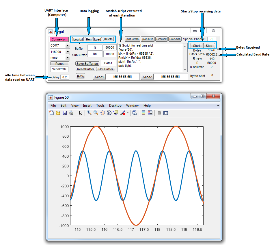
Step 4: Connect to Target
- Select COM port from dropdown (e.g., COM3, COM4)
- Set Baud rate matching UART Config block (e.g., 115200)
- Click Connect button
- Verify “Connected” status appears
- Data should start streaming immediately
Step 5: Customize Visualization
PIC GUI includes a default visualization script, but you can create custom plots:
- Click Edit Script button in PIC GUI
- Modify MATLAB code to create custom plots
- Click Start to run visualization
- Data updates in real-time as packets arrive
Example: Motor Control Data Logging
Typical use case: Monitor speed, current, and control voltage during motor operation.
Simulink Configuration
% UART Tx-Matlab block configured with 4 inputs:
% Input 1: Speed setpoint (int16, RPM)
% Input 2: Measured speed (int16, RPM)
% Input 3: Motor current (int16, mA)
% Input 4: PWM duty cycle (int16, %)
% Sample time: 1ms (1kHz data rate)
Custom Visualization Script
% Extract data from PIC GUI variables
time = data.time;
speed_ref = data.var1;
speed_meas = data.var2;
current = data.var3;
duty = data.var4;

% Create subplots
subplot(3,1,1);
plot(time, speed_ref, 'r--', time, speed_meas, 'b');
ylabel('Speed (RPM)');
legend('Reference', 'Measured');
grid on;

subplot(3,1,2);
plot(time, current, 'g');
ylabel('Current (mA)');
grid on;

subplot(3,1,3);
plot(time, duty, 'm');
ylabel('Duty Cycle (%)');
xlabel('Time (s)');
grid on;
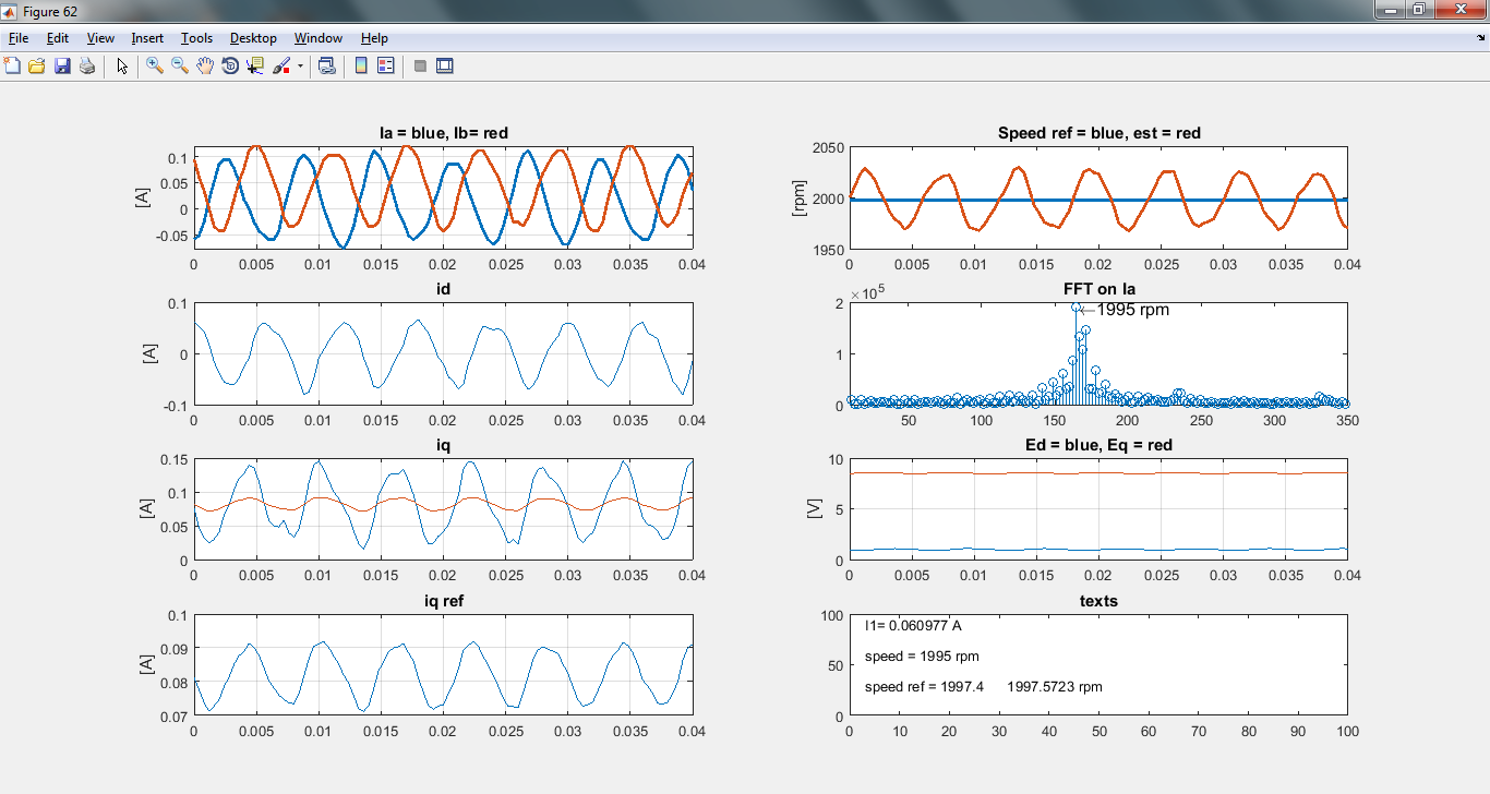
Result: Real-time plots showing motor speed tracking, current consumption, and controller output - all captured during actual hardware operation at 2000 RPM with no load.
Advanced Features
Data Logging to File
Save streamed data for offline analysis:
% In PIC GUI custom script
% Save data structure to MAT file every 10 seconds
if mod(length(data.time), 10000) == 0
    save(['motor_log_' datestr(now, 'yyyymmdd_HHMMSS') '.mat'], 'data');
end
Real-Time Signal Processing
Apply filters, FFT, or other analysis in real-time:
% Calculate moving average of current
window_size = 50;
current_filtered = movmean(data.var3, window_size);

% Compute FFT of speed signal
fs = 1000; % Sample rate (Hz)
N = length(speed_meas);
f = (0:N-1)*(fs/N);
speed_fft = abs(fft(speed_meas));

% Plot frequency spectrum
figure(2);
plot(f(1:N/2), speed_fft(1:N/2));
xlabel('Frequency (Hz)');
ylabel('Magnitude');
title('Speed Spectrum');
Automated Testing
Use PIC GUI for automated characterization:
% Run step response test automatically
% Wait for steady-state at each speed
test_speeds = [500, 1000, 1500, 2000]; % RPM
for i = 1:length(test_speeds)
    % Capture data for 5 seconds at each speed
    wait_time = 5;
    % Analyze settling time, overshoot, steady-state error
    % Save results to report
end
Multi-Variable Analysis
Correlate multiple signals to identify system behavior:
% Plot phase portrait: current vs speed
figure(3);
plot(speed_meas, current, '.');
xlabel('Speed (RPM)');
ylabel('Current (mA)');
title('Operating Point Distribution');
grid on;
Troubleshooting
No Data Received
- Check COM port: Verify correct port selected in PIC GUI (use Device Manager on Windows)
- Verify baud rate: Must match UART Config block setting exactly
- Check wiring: Ensure Tx pin of microcontroller connects to Rx of USB-Serial adapter
- Test hardware: Try loopback test (connect Tx to Rx) to verify adapter works
- Check UART pins: Verify UART Config block pin assignments match board schematic
Garbled Data / Synchronization Errors
- Baud rate mismatch: Double-check both sides set to same rate
- Buffer overflow: Reduce data rate (increase UART Tx-Matlab sample time)
- Clock accuracy: Verify oscillator configuration in Master block for accurate baud generation
- Cable quality: Use shielded USB cable, keep cable length < 3m
Slow Update Rate
- Increase baud rate: Switch from 115200 to 460800 or 2 Mbaud
- Reduce variables: Transmit fewer signals to reduce packet size
- Use integer types: int16 transmits faster than float (2 bytes vs 4 bytes)
- Increase sample time: If 1ms rate not needed, try 5ms or 10ms
- Optimize script: Reduce MATLAB processing in visualization loop
MATLAB Script Errors
- Variable naming: Use
data.var1,data.var2, etc. to access transmitted variables - Array dimensions: Check that arrays have same length before plotting
- Handle clearing: Clear figure handles properly to avoid memory leaks
- Test incrementally: Start with simple plot, add complexity gradually
Best Practices
Recommended Practices:
- Start Simple: Begin with 2-3 variables to verify communication before adding more
- Use Appropriate Data Types: int16 sufficient for most control variables, saves bandwidth
- Scale Data Properly: Apply scaling in embedded code before transmission to avoid float overhead
- Add Timestamps: Include sample counter as first variable for time-base reference
- Document Variables: Comment visualization script with variable names and units
- Save Logs: Implement automatic data saving for reproducible experiments
- Monitor Bandwidth: Calculate data rate = (bytes_per_packet × sample_rate), keep below 80% of baud rate
- Use Conditional Logging: Only transmit data when needed (e.g., when motor running)
Bandwidth Calculation Example
Ensure your data rate doesn’t exceed UART capacity:
% Configuration:
% - 5 variables (int16) = 10 bytes
% - Packet overhead (start, length, checksum) = 4 bytes
% - Total packet size = 14 bytes
% - Sample rate = 1 kHz (1ms)

bytes_per_packet = 14;
sample_rate = 1000; % Hz
data_rate = bytes_per_packet * sample_rate; % bytes/s
data_rate_bits = data_rate * 10; % 10 bits per byte (1 start + 8 data + 1 stop)

% Result: 140,000 bits/s = 140 kbps

% Check against baud rate:
baud_rate = 460800;
utilization = (data_rate_bits / baud_rate) * 100;
% Result: 30% utilization - Safe! (< 80% threshold)
Integration with Other Tools
Using PIC GUI with External Mode
Both tools can coexist if using different communication channels:
- PIC GUI: UART1 for data logging (e.g., high-speed signals)
- External Mode: UART2 for parameter tuning (e.g., PI gains)
Combining with PIL Testing
Use PIC GUI during PIL tests to capture detailed execution data:
- Run PIL test to verify algorithm correctness
- Add PIC GUI logging to same model
- Capture internal states during PIL execution
- Analyze timing, overflow conditions, state transitions
See Also
External Mode | PIL Testing | Quick Start Guide | UART Tx-Matlab Block Reference | User Guide